sd(rt(200,df = 150))[1] 1.049655sd(rnorm(200))[1] 0.9850445sd(rt(200,df = 3))[1] 1.489316Here I want to explore my intuition around standard errors where the residuals are non-normal, specifically fat-tailed.
Ordinarily a normal linear regression can be written as the following:\[ \begin{aligned} y_i \sim N(\mu_i,\sigma) \\ \mu_i = a + bx_i \end{aligned}\]
In other words the observations are modeled as if they came from a normal distribution with a mean that depends on some x value. Notably the \(\sigma\) doesn’t vary as a function of x; we assume the variance is the same for every level of x (we assume homoscedasticity). This parameter can also be called the “residual standard deviation”.
This residual standard deviation is related to how uncertain our a and b parameters are; it expresses how close to the line which OLS finds that our data is. If the data is instead fat-tailed then our residual standard error should become wider. At the edges of the distriubution our data-point’s effect on the residual is not weighted in proportion to how uncommon they are.
Let’s simulate some data, first with normal residuals and then with t-distribution (df = 4) residuals.
First let’s think through what these residuals mean. If we simulate data with rnorm() our standard deviation will by default be 1 and our mean 0. r() is will come close to this default if df is large. If df is small, the fat tails will overwhelm the computation of sd.
sd(rt(200,df = 150))[1] 1.049655sd(rnorm(200))[1] 0.9850445sd(rt(200,df = 3))[1] 1.489316The same way our standard errors for the residuals, and in turn the parameters, should grow:
x <- rnorm(200,0,1)
a <- 50
b <- 0.4
y1 <- a + b*x + rnorm(200,0,1)
y2 <- a + b*x + rt(200, df = 4)

d <- data.frame(x,y1,y2)
mdl1 <- lm(y1 ~ x, data = d)
mdl2 <- lm(y2 ~ x, data = d)

par(mfrow = c(1,2))
hist(residuals(mdl1))
hist(residuals(mdl2))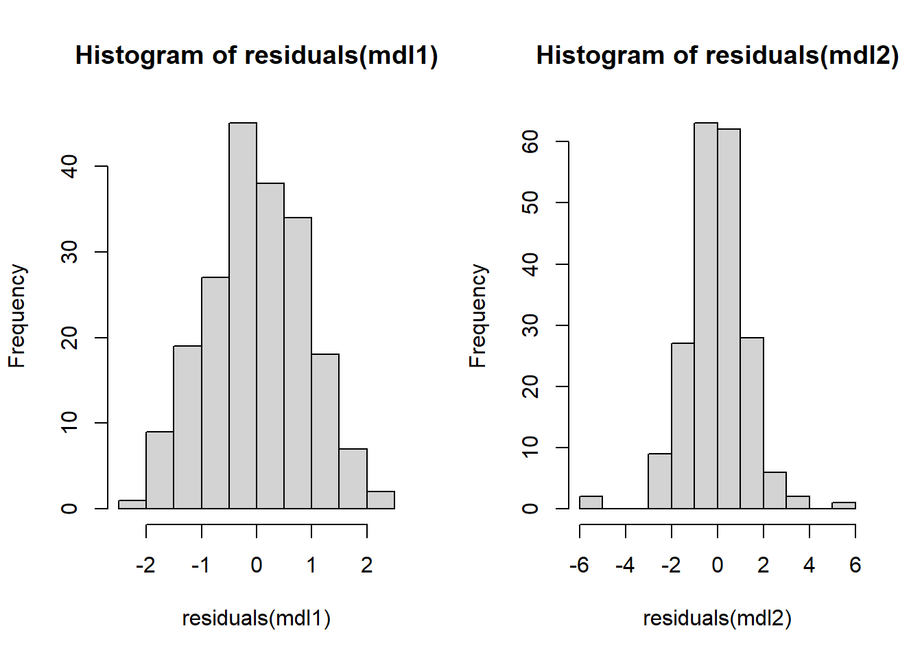
plot(x,y1)
plot(x,y2)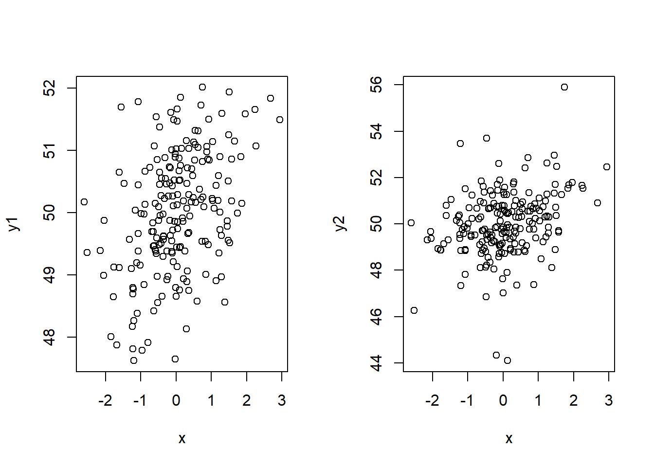
{qqnorm(residuals(mdl1))
qqline(residuals(mdl1))}

{qqnorm(residuals(mdl2))
qqline(residuals(mdl2))}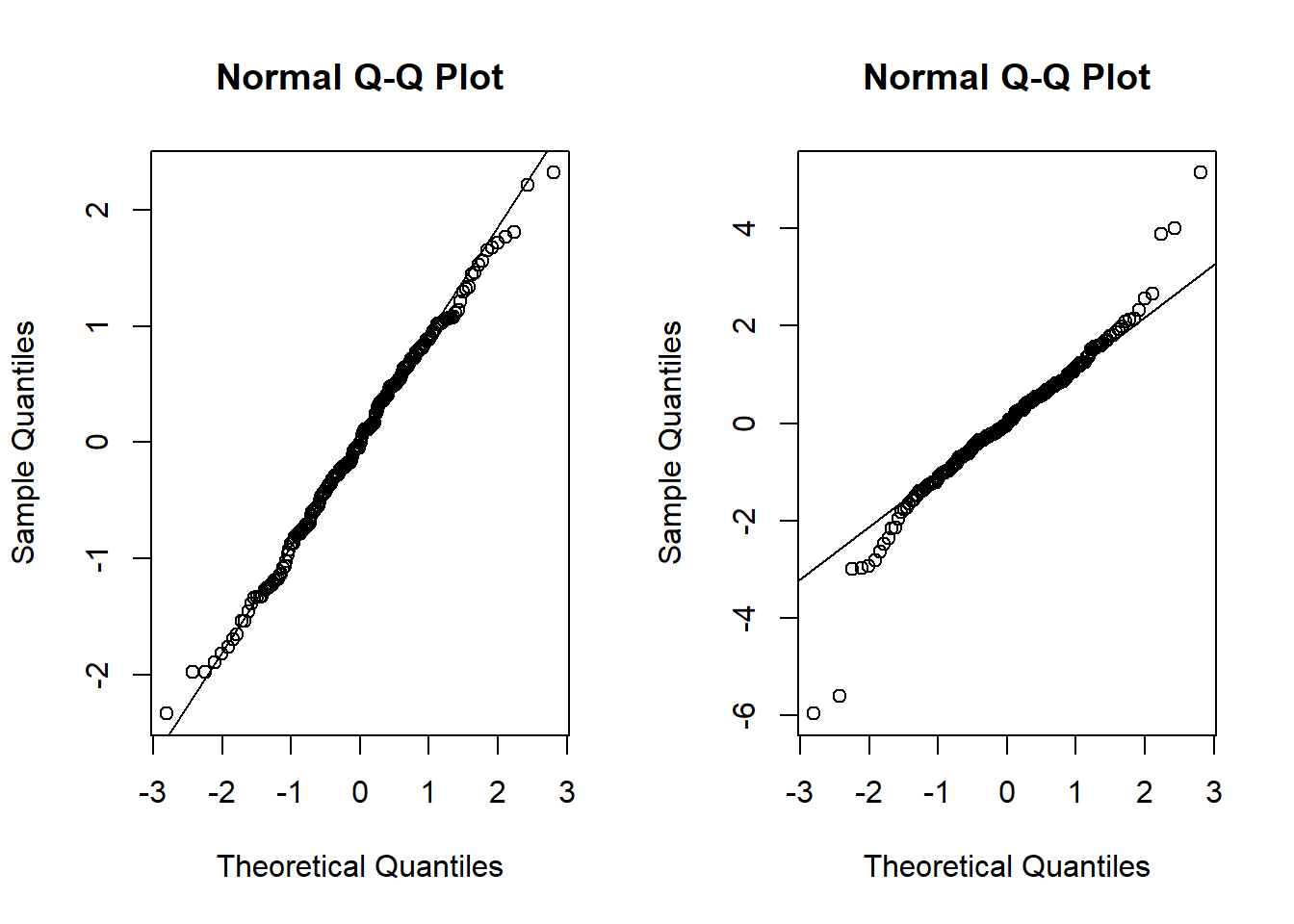
Sort of surpised the t-distribution doesn’t look worse (in a lot of runs) and the normal doesn’t look better. I guess this is good for calibrating ones expectation for how qqplots should look.
Now let’s look at the summaries of the models:
summary(mdl1)
Call:
lm(formula = y1 ~ x, data = d)

Residuals:
     Min       1Q   Median       3Q      Max
-2.33679 -0.59234 -0.01856  0.64255  2.31966

Coefficients:
            Estimate Std. Error t value Pr(>|t|)
(Intercept) 49.99326    0.06304 792.985  < 2e-16 ***
x            0.39866    0.06487   6.145 4.31e-09 ***
---
Signif. codes:  0 '***' 0.001 '**' 0.01 '*' 0.05 '.' 0.1 ' ' 1

Residual standard error: 0.8912 on 198 degrees of freedom
Multiple R-squared:  0.1602,    Adjusted R-squared:  0.1559
F-statistic: 37.77 on 1 and 198 DF, p-value: 4.306e-09summary(mdl2)
Call:
lm(formula = y2 ~ x, data = d)

Residuals:
    Min      1Q  Median      3Q     Max
-5.9553 -0.6922 -0.0218  0.7551  5.1358

Coefficients:
            Estimate Std. Error t value Pr(>|t|)
(Intercept) 49.99667    0.09625 519.435  < 2e-16 ***
x            0.43621    0.09904   4.404 1.74e-05 ***
---
Signif. codes:  0 '***' 0.001 '**' 0.01 '*' 0.05 '.' 0.1 ' ' 1

Residual standard error: 1.361 on 198 degrees of freedom
Multiple R-squared:  0.08923,   Adjusted R-squared:  0.08463
F-statistic:  19.4 on 1 and 198 DF,  p-value: 1.735e-05
This just prints one run but usually the estimate in model 2 tends to be further away from our data-generating b (which is still a true parameter) and the standard errors are (predictably) larger.
Let’s re-run it with a larger n.
x <- rnorm(10000,0,1)
a <- 50
b <- 0.4
y1 <- a + b*x + rnorm(10000,0,1)
y2 <- a + b*x + rt(10000, df = 4)

d2 <- data.frame(x,y1,y2)
mdl1b <- lm(y1 ~ x, data = d2)
mdl2b <- lm(y2 ~ x, data = d2)

summary(mdl1b)
Call:
lm(formula = y1 ~ x, data = d2)

Residuals:
    Min      1Q  Median      3Q     Max
-4.1769 -0.6783  0.0048  0.6782  3.7912

Coefficients:
            Estimate Std. Error t value Pr(>|t|)
(Intercept) 49.99796    0.01006 4968.69   <2e-16 ***
x            0.39736    0.01000   39.73   <2e-16 ***
---
Signif. codes:  0 '***' 0.001 '**' 0.01 '*' 0.05 '.' 0.1 ' ' 1

Residual standard error: 1.006 on 9998 degrees of freedom
Multiple R-squared:  0.1364,    Adjusted R-squared:  0.1363
F-statistic: 1579 on 1 and 9998 DF, p-value: < 2.2e-16summary(mdl2b)
Call:
lm(formula = y2 ~ x, data = d2)

Residuals:
     Min       1Q   Median       3Q      Max
-11.0025  -0.7472  -0.0048   0.7503  17.8787

Coefficients:
            Estimate Std. Error t value Pr(>|t|)
(Intercept) 50.01119    0.01415 3534.67   <2e-16 ***
x            0.41571    0.01406   29.56   <2e-16 ***
---
Signif. codes:  0 '***' 0.001 '**' 0.01 '*' 0.05 '.' 0.1 ' ' 1

Residual standard error: 1.415 on 9998 degrees of freedom
Multiple R-squared:  0.08039,   Adjusted R-squared:  0.0803
F-statistic:   874 on 1 and 9998 DF,  p-value: < 2.2e-16
Both estimates should now land closer, but the standard error is still larger.
So how should we think about this exercise? Do we lose power or accuracy if our data-generating process is fat-tailed and we use a normal linear regression? As far as I’ve understood, the expectation of normal residuals baked into the model risks our model getting overly influenced, sweapt away, by extreme values when estimating our b parameter.
library(robustbase)
#now using data d with n=200 again
mm_mdl2 <- lmrob(y2 ~ x, data = d, method = "MM")
summary(mdl2)
Call:
lm(formula = y2 ~ x, data = d)

Residuals:
    Min      1Q  Median      3Q     Max
-5.9553 -0.6922 -0.0218  0.7551  5.1358

Coefficients:
            Estimate Std. Error t value Pr(>|t|)
(Intercept) 49.99667    0.09625 519.435  < 2e-16 ***
x            0.43621    0.09904   4.404 1.74e-05 ***
---
Signif. codes:  0 '***' 0.001 '**' 0.01 '*' 0.05 '.' 0.1 ' ' 1

Residual standard error: 1.361 on 198 degrees of freedom
Multiple R-squared:  0.08923,   Adjusted R-squared:  0.08463
F-statistic: 19.4 on 1 and 198 DF, p-value: 1.735e-05summary(mm_mdl2)
Call:
lmrob(formula = y2 ~ x, data = d, method = "MM")
 \--> method = "MM"
Residuals:
     Min       1Q   Median       3Q      Max
-5.97953 -0.71374 -0.08105  0.76825  5.16800

Coefficients:
            Estimate Std. Error t value Pr(>|t|)
(Intercept)  50.0255     0.0821 609.326  < 2e-16 ***
x             0.4011     0.0813   4.934 1.71e-06 ***
---
Signif. codes:  0 '***' 0.001 '**' 0.01 '*' 0.05 '.' 0.1 ' ' 1

Robust residual standard error: 1.131
Multiple R-squared:  0.1065,    Adjusted R-squared:  0.102
Convergence in 7 IRWLS iterations

Robustness weights:
 2 observations c(38,48) are outliers with |weight| = 0 ( < 0.0005);
 11 weights are ~= 1. The remaining 187 ones are summarized as
    Min.  1st Qu.   Median     Mean  3rd Qu.     Max.
0.002304 0.878300 0.957300 0.900100 0.987100 0.998900
Algorithmic parameters:
       tuning.chi                bb        tuning.psi        refine.tol
        1.548e+00         5.000e-01         4.685e+00         1.000e-07
          rel.tol         scale.tol         solve.tol          zero.tol
        1.000e-07         1.000e-10         1.000e-07         1.000e-10
      eps.outlier             eps.x warn.limit.reject warn.limit.meanrw
        5.000e-04         5.352e-12         5.000e-01         5.000e-01
     nResample         max.it       best.r.s       k.fast.s          k.max
           500             50              2              1            200
   maxit.scale      trace.lev            mts     compute.rd fast.s.large.n
           200              0           1000              0           2000
                  psi           subsampling                   cov
           "bisquare"         "nonsingular"         ".vcov.avar1"
compute.outlier.stats
                 "SM"
seed : int(0)
This is just a specific run but as it turned out on my latest render we can clearly see an increase in power (here appropriate since we’ve simulated data with an effect). We can an adjusted residual standard error closer to one. On the other hand, as it turned out the estimate didn’t actually land closer to the data-generating input. I’d guess that it does if we scale it though.
Note that there are many other robust regression methods that could be appropriate here.
I’ve not gotten into the weeds of that MM estimation does, but from what I’ve read it’s flexible and usually good. It doesn’t go awry when there are no outliers but are also not mislead by outliers.